torch_study_1
"/home/yossef/notes/personal/ml/torch_study/torch_study_1.md"
path: personal/ml/torch_study/torch_study_1.md
- **fileName**: torch_study_1
- **Created on**: 2026-04-02 19:00:36
## making some imports

import torch
import torch.nn as nn
import torch.optim as optim

# less random for hte application data when genertated too showiong hte same results each time
torch.manual_seed(1)
<torch._C.Generator at 0x7f72ffcd6450>
destances = torch.tensor([[1.0], [2.0], [3.0], [4.0]], dtype=torch.float)
times = torch.tensor([[6.96], [12.11], [16.77], [22.21]], dtype=torch.float)
# so this meaning that the model gone taking only one feature input and output only one output 1,1
model = nn.Sequential(nn.Linear(1, 1))
so now what after creating hte mode
need too understand hte model output too find if it's good or bad so
gone understand the model by check for one things
- the output for the model if it's good or bad based on the calc hte loss for hte model so this made by having two sets of data one is train data and another is test data so after the model is trained so now
there is a idea tooo get a data that u have the right answer for it
and then making hte model test this data (but don't see the answers at
all) so now after that now hte model preduce or output the answer for
the datta now chcek for this datta if it's right or wrong this by calc
the less function for this by nn.(losses functions)
and after that gone making optimzer for hte model that this mean so
now i have the error value (precent for the data) so gone try too
making a gradent descent getting the best value for weight and bais
for the model too making the model smarter and less error using this
loss_function = nn.MSELoss()
# so what is the lr -> learing rate for the model it's how every time the value for the model when lrean (how much increase or decrease)
optimzer = optim.SGD(model.parameters(), lr=0.1)
from torch.nn.modules import distance
for epochs in range(500):
    optimzer.zero_grad()

    outputs = model(destances)

    loss = loss_function(outputs, times)
    loss.backward()

    optimzer.step()
import torch
import matplotlib.pyplot as plt
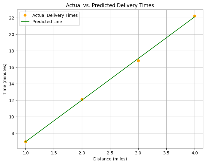
def plot_results(model, distances, times):
"""
Plots the actual data points and the model's predicted line for a given dataset.
Args:
model: The trained machine learning model to use for predictions.
distances: The input data points (features) for the model.
times: The target data points (labels) for the plot.
"""
# Set the model to evaluation mode
model.eval()
# Disable gradient calculation for efficient inference
with torch.no_grad():
# Make predictions using the trained model
predicted_times = model(distances)
# Create a new figure for the plot
plt.figure(figsize=(8, 6))
# Plot the actual data points
plt.plot(distances.numpy(), times.numpy(), color='orange', marker='o', linestyle='None', label='Actual Delivery Times')
# Plot the predicted line from the model
plt.plot(distances.numpy(), predicted_times.numpy(), color='green', marker='None', label='Predicted Line')
# Set the title of the plot
plt.title('Actual vs. Predicted Delivery Times')
# Set the x-axis label
plt.xlabel('Distance (miles)')
# Set the y-axis label
plt.ylabel('Time (minutes)')
# Display the legend
plt.legend()
# Add a grid to the plot
plt.grid(True)
# Show the plot
plt.show()
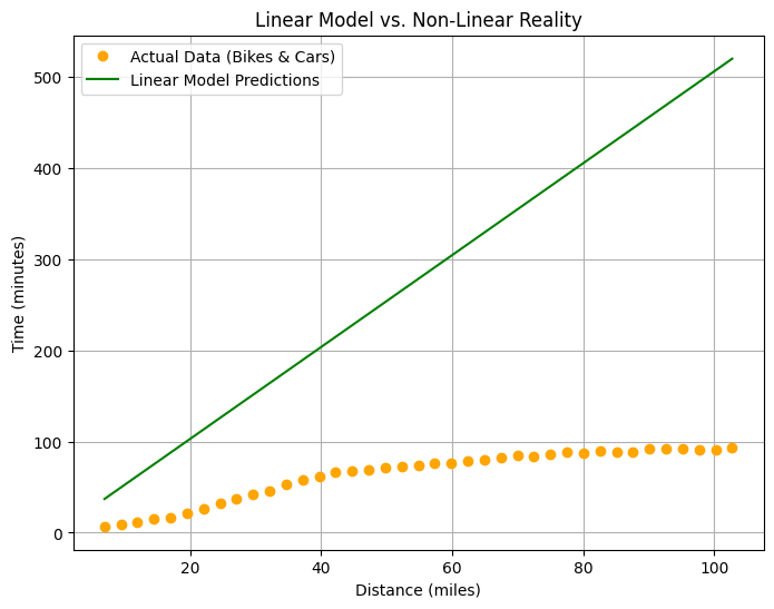
def plot_nonlinear_comparison(model, new_distances, new_times):
"""
Compares and plots the predictions of a model against new, non-linear data.
Args:
model: The trained model to be evaluated.
new_distances: The new input data for generating predictions.
new_times: The actual target values for comparison.
"""
# Set the model to evaluation mode
model.eval()
# Disable gradient computation for inference
with torch.no_grad():
# Generate predictions using the model
predictions = model(new_distances)
# Create a new figure for the plot
plt.figure(figsize=(8, 6))
# Plot the actual data points
plt.plot(new_distances.numpy(), new_times.numpy(), color='orange', marker='o', linestyle='None', label='Actual Data (Bikes & Cars)')
# Plot the predictions from the model
plt.plot(new_distances.numpy(), predictions.numpy(), color='green', marker='None', label='Linear Model Predictions')
# Set the title of the plot
plt.title('Linear Model vs. Non-Linear Reality')
# Set the label for the x-axis
plt.xlabel('Distance (miles)')
# Set the label for the y-axis
plt.ylabel('Time (minutes)')
# Add a legend to the plot
plt.legend()
# Add a grid to the plot for better readability
plt.grid(True)
# Display the plot
plt.show()
plot_results(model, destances, times)
new_destance = torch.tensor([7.0], dtype = torch.float)
## so now we want too maknig a predection this this value

# 7 * 12 / 2 = 42

with torch.no_grad():
    new_prediected_time = model(new_destance)
print(f"the new time is: ${new_prediected_time}")
the new time is: $tensor([37.1970])
model
Sequential( (0): Linear(in_features=1, out_features=1, bias=True) )
model[0]
Linear(in_features=1, out_features=1, bias=True)
layer = model[0]
weight = layer.weight.data.numpy()
bias = layer.bias.data.numpy()
print(f"the weight is: {weight}")
print(f"the bias is: {bias}")
the weight is: 5.041001 the bias is: [1.9099984]
# time = 5.0 * Distance + 2.0
# ?? = 5.0 * 2 + 2 ====== 12
# 5.0 * 7 + 2 ===== 37
# y = wx + b
# w => weight , b => bias
so now gone try too adding more complex strcture data
so now gone using more data for bikes and cars for the new destances
and the times for the treval so gone see if the model gone find and
understand this new data or not
new_distances_data = torch.tensor([
    [1.0], [1.5], [2.0], [2.5], [3.0], [3.5], [4.0], [4.5], [5.0], [5.5],
    [6.0], [6.5], [7.0], [7.5], [8.0], [8.5], [9.0], [9.5], [10.0], [10.5],
    [11.0], [11.5], [12.0], [12.5], [13.0], [13.5], [14.0], [14.5], [15.0], [15.5],
    [16.0], [16.5], [17.0], [17.5], [18.0], [18.5], [19.0], [19.5], [20.0]
], dtype=torch.float)
new_times_data = torch.tensor([
    [6.96], [9.67], [12.11], [14.56], [16.77], [21.7], [26.52], [32.47], [37.15], [42.35],
    [46.1], [52.98], [57.76], [61.29], [66.15], [67.63], [69.45], [71.57], [72.8], [73.88],
    [76.34], [76.38], [78.34], [80.07], [81.86], [84.45], [83.98], [86.55], [88.33], [86.83],
    [89.24], [88.11], [88.16], [91.77], [92.27], [92.13], [90.73], [90.39], [92.98]
], dtype=torch.float)
now lets test the model with the new data and see how it's gone performance
## so torch no_grad tell the kernal for torch don't make all the complex operation like on train
## it's just gone predection this new predection data not making a full train again so for making
## the predection faster and not using a lot of resourses

with torch.no_grad():
    new_output = model(new_distances_data)
now calc the loss andd optimizer for get the right value for weight and bias for model
new_loss = loss_function(new_output, new_times_data)
print(f"the new loss function {new_loss.item():.2f}")
the new loss function 176.32
so from the output for loss it's tooo high this mean it's tooo bad for the model too making a prediection for data that having bike and cars so whyyyyyyyyyyyyyyyyyyyyyyyyyyyyyyyy
- on the first train model u making a predection between the time and
distance that what the model train on so for example if the distance
high the time gone be high make sence ;))))))))) but now u having tooo
subset of data the linear equation not gone handle because
if the bike distance for example is 4mile and it's taking it on 20
mintes does the car gone having the same time on the 4 mile
so the equation was ( y = wx+b + but must adding more and more
feature for more details for the model too understand what we want too
do and making a prediction rights : ((( transpert type => car, bike
))) + road type (stright, cerves) + weather type + car type IF CAR
ONLY OFFCOURSE , traffic status today
plot_nonlinear_comparison(model, new_output, new_times_data)
before:./helper_utils.md
continue:torch_study_2